Introduction

In our recent AI-revolutionized world, to design proper machine learning workflows is important for getting insights, making predictions, and also solving complex problems. Python, with its vast collection of libraries and frameworks, is the go-to language for developing machine learning models and workflows. So, that's why, understanding the steps involved in designing machine learning workflows in Python is essential to progress in this field.

In this article, we will explore the fundamental steps and considerations that go into building efficient and robust machine learning pipelines. We will cover all the essential aspects that is needed using some of the extensive support from libraries such as NumPy, Pandas, Scikit-Learn, TensorFlow, and PyTorch.

So, let's dive in and discover the key components of designing machine learning workflows in Python. By the end of this article, you'll have a solid foundation to tackle real-world machine learning challenges and unleash the power of Python in your data-driven endeavors.

What's the process?

To design a machine learning workflow, we have to perform and maintain some specific steps which are crucial. They are stated below:

1. Data Preparation

   It is a crucial step in designing machine learning workflows. It involves ensuring that the data is in a suitable format and quality for the subsequent stages of the workflow.

# Import necessary libraries
import numpy as np
import pandas as pd

# Load and explore the dataset
dataset = pd.read_csv('data.csv')
print(dataset.head())

# Handle missing data and outliers
dataset = dataset.dropna()
dataset = dataset[dataset['column'] < threshold]

# Preprocess the data
X = dataset.drop('target', axis=1)
y = dataset['target']

# Split the data into training and testing sets
from sklearn.model_selection import train_test_split
X_train, X_test, y_train, y_test = train_test_split(X, y, test_size=0.2)

1. Feature Engineering

   It is the next step that comes after Data Preparation. It involves transforming raw data into a format that can effectively represent the underlying patterns and relationships in them.

# Extract relevant features from the data
# Feature extraction techniques like PCA, LDA, etc.

# Perform dimensionality reduction
from sklearn.decomposition import PCA
pca = PCA(n_components=2)
X_train_pca = pca.fit_transform(X_train)
X_test_pca = pca.transform(X_test)

1. Model Selection

   The model selection section involves choosing an appropriate algorithm or model architecture that best fits the problem at hand. It includes tasks such as determining the type of problem selecting the appropriate model class (e.g., decision trees, neural networks, support vector machines), and tuning hyperparameters to optimize model performance.

# Import necessary libraries
from sklearn.model_selection import cross_val_score
from sklearn.metrics import accuracy_score, precision_score, recall_score

# Choose appropriate models based on the problem
from sklearn.linear_model import LogisticRegression
from sklearn.ensemble import RandomForestClassifier

# Split data into input features (X) and target variable (y)
X = X_train_pca
y = y_train

# Define evaluation metrics for model selection
scoring = 'accuracy'

# Train and evaluate models using cross-validation
model_lr = LogisticRegression()
scores_lr = cross_val_score(model_lr, X, y, cv=5, scoring=scoring)
model_rf = RandomForestClassifier()
scores_rf = cross_val_score(model_rf, X, y, cv=5, scoring=scoring)

# Select the best-performing model based on evaluation metrics
best_model = model_rf if np.mean(scores_rf) > np.mean(scores_lr) else model_lr

1. Model Training and Evaluation

   The model training process involves feeding the input data and corresponding labels into the model, adjusting the model's internal parameters iteratively using optimization techniques (e.g., gradient descent), and updating the parameters to minimize the specified loss function. Evaluation metrics such as accuracy, precision, recall, or mean squared error are calculated to quantify the model's predictive performance.

# Train the selected model on the training set
best_model.fit(X_train_pca, y_train)

# Evaluate the model using test set
y_pred = best_model.predict(X_test_pca)

# Calculate evaluation metrics
accuracy = accuracy_score(y_test, y_pred)
precision = precision_score(y_test, y_pred)
recall = recall_score(y_test, y_pred)

1. Model Deployment

   The Model Deployment section involves making the trained machine learning model available for use in real-world applications. This process includes preparing the model for deployment, such as converting it into a deployable format or packaging it into a containerized environment.

# Save the trained model to a file
import joblib
joblib.dump(best_model, 'model.pkl')

Now, with all these covered, it may seem overwhelming to you, so let’s check some examples to solidify your concepts.

Examples

Machine Learning workflow for Image Classification using the Fashion MNIST dataset

Here's an example of a machine learning workflow for image classification using the Fashion MNIST dataset. The workflow includes data loading, preprocessing, model selection, training, evaluation, and saving the trained model. Let’s check the code sample, how we are doing that-

# Import necessary libraries
import tensorflow as tf
from tensorflow import keras
import numpy as np

# Load the Fashion MNIST dataset
fashion_mnist = keras.datasets.fashion_mnist
(X_train, y_train), (X_test, y_test) = fashion_mnist.load_data()

# Preprocess the data
X_train = X_train / 255.0
X_test = X_test / 255.0

# Model Selection
model = keras.models.Sequential([
    keras.layers.Flatten(input_shape=(28, 28)),
    keras.layers.Dense(128, activation='relu'),
    keras.layers.Dense(10, activation='softmax')
])

# Model Training
model.compile(optimizer='adam', loss='sparse_categorical_crossentropy', metrics=['accuracy'])
model.fit(X_train, y_train, epochs=10)

# Model Evaluation
test_loss, test_accuracy = model.evaluate(X_test, y_test)
print(f"Test Loss: {test_loss}")
print(f"Test Accuracy: {test_accuracy}")

# Save the trained model
model.save("fashion_mnist_model.h5")

Now, let’s see how the workflow works:

1. We import the necessary libraries, including TensorFlow and Keras, which provide high-level APIs for building and training deep learning models.

2. The Fashion MNIST dataset is loaded using the keras.datasets.fashion_mnist module and is split into training and testing sets, and the images and labels are stored in variables X_train, y_train, X_test, and y_test, respectively.

3. Pre-processing the data: The pixel values of the images are scaled to a range of 0 to 1 by dividing them by 255. This normalization step ensures that the input data is in a suitable range for the model.

4. Model Selection: We create a sequential model using keras.models.Sequential(). In this example, we use a simple architecture with a flattening layer, a dense layer with 128 units and ReLU activation, and a dense output layer with 10 units (corresponding to the number of classes in the dataset) and softmax activation.

5. Model Training: We compile the model using model.compile() with the Adam optimizer, sparse categorical cross-entropy loss function, and accuracy as the evaluation metric. The model is trained using model.fit() with the training data (X_train and y_train) for a specified number of epochs.

6. Model Evaluation: We evaluate the trained model on the test set using model.evaluate(). The test loss and accuracy are calculated and printed.

Saving the trained model: We save the trained model to a file using model.save().

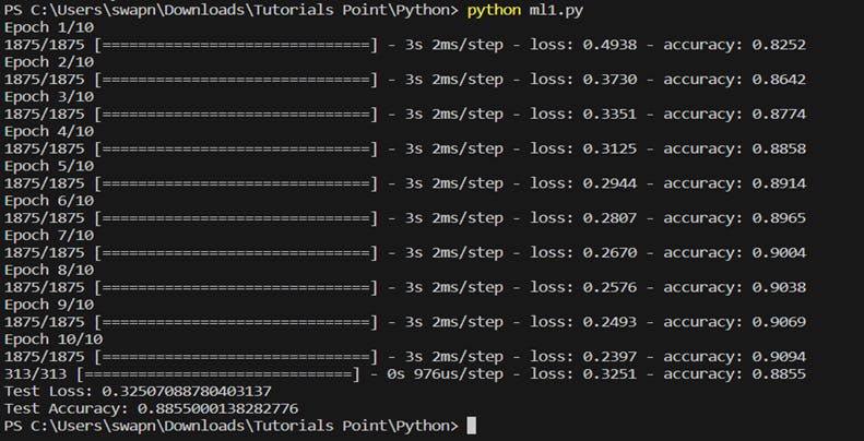
When the code is run through the terminal, the model is trained, evaluated and the test loss and accuracy is printed, as shown below:

Machine Learning workflow for Sentiment Analysis using the IMDb movie review dataset

Let’s get into the example of a machine learning workflow for sentiment analysis using the IMDb movie review dataset. The workflow includes data preparation, feature engineering, model selection, training, evaluation, and deployment. Let’s dive into the code and check how we are doing that-

# Import necessary libraries
import pandas as pd
from sklearn.feature_extraction.text import TfidfVectorizer
from sklearn.model_selection import train_test_split
from sklearn.linear_model import LogisticRegression
from sklearn.metrics import accuracy_score
import joblib

# Load the IMDb movie review dataset
df = pd.read_csv('imdb_reviews.csv')

# Data Preparation
X = df['review']
y = df['sentiment']

# Split the data into training and testing sets
X_train, X_test, y_train, y_test = train_test_split(X, y, test_size=0.2, random_state=42)

# Feature Engineering
vectorizer = TfidfVectorizer()
X_train_vectors = vectorizer.fit_transform(X_train)
X_test_vectors = vectorizer.transform(X_test)

# Model Selection
model = LogisticRegression(max_iter=100000)

# Model Training
model.fit(X_train_vectors, y_train)

# Model Evaluation
y_pred = model.predict(X_test_vectors)
accuracy = accuracy_score(y_test, y_pred)
print(f"Accuracy: {accuracy}")

# Model Deployment
joblib.dump(model, 'sentiment_analysis_model.pkl')
joblib.dump(vectorizer, 'vectorizer.pkl')

Now, let’s see how the workflow works:

1. We start by importing the necessary libraries, including Pandas for data manipulation, scikit-learn for machine learning functionality, and joblib for model serialization.

2. The IMDb movie review dataset is loaded using pd.read_csv() into a Pandas DataFrame called df. The dataset contains two columns: "review" (textual movie reviews) and "sentiment" (positive or negative sentiment).

3. Data Preparation: We assign the "review" column to X and the "sentiment" column to Y, which prepares the data for training and testing.

4. Splitting the data: The train_test_split() function is used to split the data into training and testing sets. We assign 80% of the data to training and 20% to testing. The random_state parameter ensures reproducibility of the split.

5. Feature Engineering: We use the TfidfVectorizer from scikit-learn to convert the textual reviews into numerical features. The fit_transform() function is applied to the training set (X_train), and the transform() function is applied to the testing set (X_test), as you can clearly see in the code.

6. Model Selection: We choose a logistic regression model for sentiment analysis. In this example, we use scikit-learn's LogisticRegression() class.

7. Model Training: We fit the logistic regression model to the training data using model.fit() with the training vectors (X_train_vectors) and corresponding labels (y_train).

8. Model Evaluation: We make predictions on the testing set using model.predict() with the testing vectors (X_test_vectors). The accuracy is calculated by comparing the predicted labels (y_pred) with the actual labels (y_test).

9. Model Deployment: And finally, we save the trained model and vectorizer using joblib.dump() for future use and deployment.

When the code is run through the terminal, the model is trained, evaluated and the accuracy is printed, as shown below:

Conclusion

Thank you for reading the blog! I hope you found it informative and valuable. For more information, follow me on Twitter (swapnoneel123) where I share more such content through my tweets and threads. And, please consider sharing it with others on Twitter and tag me in your post so I can see it too. You can also check my GitHub (Swpn0neel) to see my projects.

I wish you a great day ahead and till then keep learning and keep exploring!!